2.2 Model Mechanics

1. Fundamental Mechanics

The cost function and the 1st order optimization method used in Logistic Regression since there is no close form solution.

1.1 Cost Function in Logistic Regression

In logistic regression, we predict probabilities using the sigmoid function:

where represents the parameters, and represents the feature vector.

The cost function for logistic regression is the log loss (cross-entropy loss):

where:

• is the number of training examples.
• is the actual label (0 or 1).
• is the predicted probability.

This function measures how well our logistic regression model fits the data. Our goal is to minimize .

1.2 Gradient Descent for Logistic Regression

Gradient descent is an optimization algorithm used to find the optimal parameters that minimize the cost function.

Steps of Gradient Descent:

1. Compute the gradient (partial derivative of cost function w.r.t ):

   This represents how much the cost function changes with respect to each parameter .

2. Update the parameters using the learning rate :

   for all , where is the number of features.

3. Repeat until convergence: Iterate over the dataset multiple times until stabilizes (i.e., changes very little between iterations).

Key Considerations

• Learning Rate (): If is too large, gradient descent may overshoot the minimum; if too small, convergence will be slow.
• Feature Scaling: Standardizing features (e.g., using mean normalization) can speed up convergence.
• Stopping Criteria: Stop when the change in is below a small threshold or after a fixed number of iterations.

2. Gradient Calculation of LR

Following shows the step by step to derive the gradient of the cost function in logistic regression.

Step 1: Define the Cost Function

The logistic regression cost function is given by:

where:

• is the sigmoid function:

• is the number of training examples.

• is the actual label (0 or 1).

• is the feature vector for the -th training example.

Step 2: Compute the Partial Derivative

We need to compute the derivative of with respect to :

Step 2.1: Differentiate the Cost Function

Rewriting the cost function:

Differentiating both sides:

Step 2.2: Compute

We use the sigmoid function:

Differentiating w.r.t :

Step 2.3: Substitute Back

Substituting this into our gradient equation:

Canceling terms:

Factor out :

Since , we get:

Final Gradient Descent Update Rule

Using gradient descent:

where:

• is the learning rate.

Summary

1. We computed the cost function .

2. We found its derivative w.r.t. .

3. We obtained the final gradient formula:

4. We use this in gradient descent to update .

Code

import numpy as np
import matplotlib.pyplot as plt

def sigmoid(z):
    return 1 / (1 + np.exp(-z))

def compute_cost(X, y, theta):
    m = len(y)
    h = sigmoid(X @ theta)
    cost = (-1/m) * np.sum(y * np.log(h) + (1 - y) * np.log(1 - h))
    return cost

def gradient_descent(X, y, theta, alpha, iterations):
    m = len(y)
    cost_history = []

    for _ in range(iterations):
        h = sigmoid(X @ theta)
        gradient = (1/m) * (X.T @ (h - y))
        theta -= alpha * gradient
        cost_history.append(compute_cost(X, y, theta))

    return theta, cost_history

# Example usage
np.random.seed(42)
m, n = 100, 2  # 100 samples, 2 features
X = np.random.rand(m, n)
y = (X[:, 0] + X[:, 1] > 1).astype(int).reshape(-1, 1)  # Simple linear decision boundary

# Add intercept term (bias)
X = np.c_[np.ones((m, 1)), X]  # Add a column of ones for the bias term

theta = np.zeros((n + 1, 1))  # Initialize theta with zeros
alpha = 0.1
iterations = 1000

# Train logistic regression model
theta_optimal, cost_history = gradient_descent(X, y, theta, alpha, iterations)

# Plot cost function convergence
plt.plot(range(iterations), cost_history, label='Cost Function')
plt.xlabel('Iterations')
plt.ylabel('Cost')
plt.title('Cost Function Convergence')
plt.legend()
plt.show()

print("Optimal theta:", theta_optimal)

Explanation

1. Sigmoid Function: Implements .
2. Compute Cost: Implements the cost function .
3. Gradient Descent: Updates iteratively using the derived formula.
4. Data Generation: Creates synthetic data where the sum of two features determines the class.
5. Model Training: Runs gradient descent and prints the optimal .

3. Convexity of the Cost Function

The cost function of logistic regression is convex. This is a crucial property because convexity ensures that optimization algorithms like Gradient Descent can efficiently find the global minimum without getting stuck in local minima.

3.1 Why is the Cost Function Convex?

Logistic regression uses the log-loss (binary cross-entropy loss) as its cost function:

where:

• is the sigmoid function (hypothesis).
• is the actual label ( or ).
• is the input feature vector.
• represents the model parameters.

3.2 Proof of Convexity (Intuition)

1. Sigmoid Function Properties: The sigmoid function is convex and concave (S-shape), but when combined with the log function in the loss function, the overall cost function remains convex.
2. Second Derivative Analysis: The Hessian matrix (second derivative of ) is positive semi-definite, which confirms convexity.
3. Gradient Descent Works Well: Since the cost function is convex, Gradient Descent always converges to the global minimum, unlike non-convex functions, which may have multiple local minima.

IMPORTANT

✅ Convexity ensures global optimality in logistic regression.
✅ Gradient Descent is guaranteed to converge (with a suitable learning rate).
✅ Regularization (L1/L2) does not change convexity—it just reshapes the loss surface.

3.3 Close Form Solution ?

The cost function of logistic regression does not have a closed-form solution due to the non-linearity introduced by the sigmoid function in the hypothesis.

1. Logistic Regression Hypothesis: The logistic regression model is defined as:

   This is a sigmoid function, which transforms the linear combination of features into a probability between 0 and 1.

2. Log-Loss (Binary Cross-Entropy) Cost Function: The cost function for logistic regression is:

   This is a sum of logarithms involving , which itself includes the sigmoid function.

3. Lack of Closed-Form Solution:

   • The derivative of the sigmoid function involves terms that make the cost function non-linear with respect to .
   • Specifically, the logarithm of the sigmoid function creates a function that cannot be simplified into a closed-form algebraic solution for .
   • Closed-form solutions (like in linear regression) arise when the cost function is quadratic, meaning it is a parabola or some simple geometric shape where the minimum is easily solvable using algebra (e.g., by setting the gradient equal to zero).
   • In logistic regression, the non-linear combination of the sigmoid function with the log-likelihood doesn’t allow for a simple algebraic solution.

Why Can’t We Solve It Algebraically?

The process of minimizing the cost function for logistic regression requires numerical optimization methods (like Gradient Descent) because the cost function is non-convex and not expressible in closed-form.

If we attempt to differentiate the cost function, we get a complicated expression that still requires iterative methods like gradient descent to find the minimum.

IMPORTANT

• Linear regression has a closed-form solution because its cost function is quadratic, leading to a simple algebraic solution.
• Logistic regression, with its logistic (sigmoid) function and logarithmic cost function, doesn’t have a closed-form solution because the optimization involves non-linear terms that can’t be simplified algebraically.

What We Use Instead

• Gradient Descent: An iterative optimization method used to find the minimum of the cost function.
• Newton’s Method (or variants like L-BFGS): More advanced methods that improve the efficiency of optimization.

4. Formulation of the Kernel Trick

In the original space, SVM seeks to find the optimal hyperplane that maximizes the margin:

Where:

• is the weight vector.
• is the bias term.
• is the data point.
• is the class label.

In the kernel trick, instead of working directly in the original space, we use a kernel function to compute the inner product in the transformed feature space. This kernel function computes:

Where represents the transformation to the higher-dimensional space.

The kernel trick allows us to compute the dot product in the higher-dimensional space without explicitly transforming the data.

4.1 Common Kernel Functions

1. Linear Kernel:

   • Equivalent to no transformation (works for linearly separable data).

2. Polynomial Kernel:

   • Transforms the data to a higher-degree polynomial space. This can create curved decision boundaries.

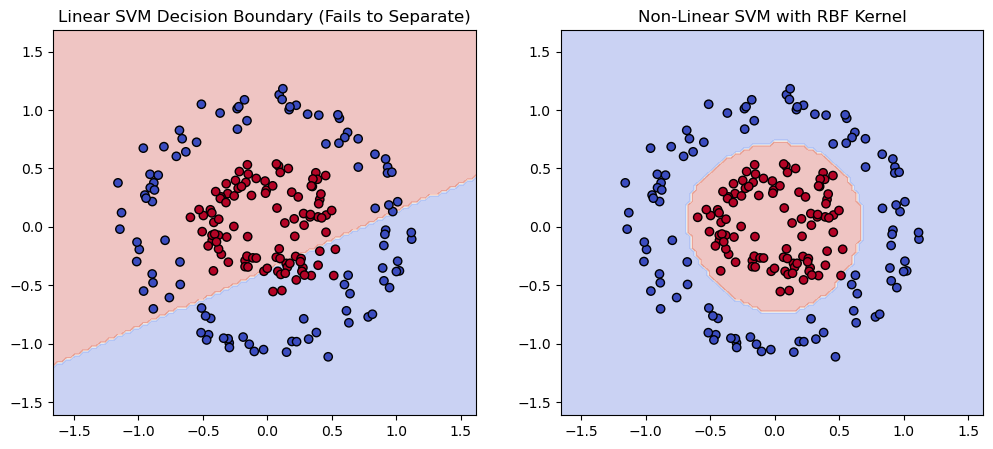
3. Radial Basis Function (RBF) Kernel (Gaussian Kernel):

   • This is the most popular kernel, which maps the data into an infinite-dimensional space. It allows SVMs to create highly flexible, non-linear decision boundaries.

4. Sigmoid Kernel:

   • Similar to neural networks’ activation functions.

4.2 Code

# Generate synthetic non-linearly separable dataset (circles)
from sklearn.datasets import make_circles
from sklearn.svm import SVC
import matplotlib.pyplot as plt
import numpy as np

# Create a dataset with concentric circles
X_circles, y_circles = make_circles(n_samples=200, noise=0.1, factor=0.4, random_state=42)

# Train a linear SVM (for comparison)
svm_linear = SVC(kernel="linear")
svm_linear.fit(X_circles, y_circles)

# Train an RBF SVM (non-linear kernel)
svm_rbf = SVC(kernel="rbf", gamma="scale")
svm_rbf.fit(X_circles, y_circles)

# Create a mesh grid for visualization
x_min, x_max = X_circles[:, 0].min() - 0.5, X_circles[:, 0].max() + 0.5
y_min, y_max = X_circles[:, 1].min() - 0.5, X_circles[:, 1].max() + 0.5
xx, yy = np.meshgrid(np.linspace(x_min, x_max, 100), np.linspace(y_min, y_max, 100))

# Predict decision boundaries
Z_linear = svm_linear.predict(np.c_[xx.ravel(), yy.ravel()]).reshape(xx.shape)
Z_rbf = svm_rbf.predict(np.c_[xx.ravel(), yy.ravel()]).reshape(xx.shape)

# Plot the results
plt.figure(figsize=(12, 5))

# Linear SVM decision boundary
plt.subplot(1, 2, 1)
plt.contourf(xx, yy, Z_linear, alpha=0.3, cmap='coolwarm')
plt.scatter(X_circles[:, 0], X_circles[:, 1], c=y_circles, edgecolor='k', cmap='coolwarm')
plt.title("Linear SVM Decision Boundary (Fails to Separate)")

# Non-linear SVM decision boundary (RBF Kernel)
plt.subplot(1, 2, 2)
plt.contourf(xx, yy, Z_rbf, alpha=0.3, cmap='coolwarm')
plt.scatter(X_circles[:, 0], X_circles[:, 1], c=y_circles, edgecolor='k', cmap='coolwarm')
plt.title("Non-Linear SVM with RBF Kernel")

plt.show()