2.1 Fundamentals

1. Definition

1.1 What is a Classification Problem?

A classification problem is a type of supervised learning task where the goal is to assign inputs to discrete categories or classes. The model learns from labeled training data and predicts the class of new data points.

Classification problems typically involve:

1. Discrete outputs (e.g., categories like “spam” or “not spam”).
2. Decision boundaries that separate different classes.
3. Probabilistic predictions, often using algorithms like logistic regression, decision trees, SVMs, or deep learning models.

1.2 Examples of Classification Problems

1. Binary Classification (Two Classes)

• Email spam detection (Spam or Not Spam)
• Credit card fraud detection (Fraudulent or Legitimate Transaction)
• Disease diagnosis (Diseased or Healthy)
• Customer churn prediction (Will leave or Will stay)

2. Multiclass Classification (More than Two Classes)

• Handwritten digit recognition (Digits 0-9)
• Sentiment analysis (Positive, Neutral, or Negative Review)
• Species classification (Dog, Cat, or Bird)
• Product recommendation (Electronics, Clothing, or Books)

3. Multi-label Classification (One Sample Belongs to Multiple Classes)

• Image tagging (A photo may contain a “cat” and a “tree” simultaneously)
• News categorization (An article may belong to “Politics” and “Economy”)
• Medical diagnosis (A patient may have both “Diabetes” and “Hypertension”)

1.3 Common Algorithms for Classification

• Logistic Regression (for binary classification)
• Decision Trees & Random Forests
• Support Vector Machines (SVM)
• Naïve Bayes
• Neural Networks & Deep Learning (e.g., CNNs for image classification)

2. Logistic regression vs Linear Regression

Logistic regression and linear regression differ in several key aspects, including the type of data they handle, the model they use, the loss function, and the optimization process. Here’s a detailed comparison:

2.1 Data Type

• Linear Regression: Used for continuous dependent variables (e.g., predicting house prices, salaries).
• Logistic Regression: Used for categorical (typically binary) dependent variables (e.g., classifying emails as spam or not spam).

2.2 Model (Hypothesis Function)

• Linear Regression: Models the relationship between the input features and the output as a linear function:
• Logistic Regression: Uses a sigmoid function (logistic function) to transform the output into a probability: This ensures that the output is between 0 and 1, making it suitable for classification.

2.3 Loss Function

• Linear Regression: Uses Mean Squared Error (MSE):
• Logistic Regression: Uses Log-Loss (Binary Cross-Entropy): This loss is more appropriate for classification since it penalizes incorrect class probabilities more effectively.

2.4 Optimization Algorithm

• Linear Regression: Can be solved using Ordinary Least Squares (OLS) (closed-form solution) or Gradient Descent.
• Logistic Regression: No closed-form solution exists, so optimization is done using Gradient Descent or variants like Stochastic Gradient Descent (SGD), Newton’s Method, or L-BFGS.

2.5 Output Interpretation

• Linear Regression: Directly predicts the output .
• Logistic Regression: Predicts a probability, which is then thresholded (typically at 0.5) to determine the class label.

Summary

Feature	Linear Regression	Logistic Regression
Target Variable	Continuous	Binary/Categorical
Model Equation		Logistic Cost Ref 2.2
Loss Function	Mean Squared Error (MSE)	Log Loss (Binary Cross-Entropy)
Optimization	OLS or Gradient Descent	Gradient Descent (or other methods)
Output	Real value ()	Probability (0 to 1)
Interpretation	Direct prediction	Probability-based classification

3. Intuition Behind SVM

3.1 Intuition Behind Support Vector Machines (SVMs)

Support Vector Machines (SVMs) are designed to find the optimal decision boundary that best separates different classes in a dataset. The key intuition is:

1. Maximizing the Margin: Instead of just finding any decision boundary like logistic regression, SVM aims to find the widest possible margin between two classes. This margin is the distance between the closest data points (called support vectors) and the decision boundary (hyperplane).

2. Robustness: By maximizing the margin, SVM generalizes better and avoids overfitting, especially in high-dimensional spaces.

3. Handling Non-Linearity: If the data is not linearly separable, SVM uses the kernel trick to transform the data into a higher-dimensional space where it becomes separable.

3.2 How SVM Differs from Logistic Regression

Feature	Logistic Regression	Support Vector Machine (SVM)
Objective	Minimize log-loss (maximize likelihood)	Maximize the margin between classes
Decision Boundary	Soft boundary, probability-based	Hard boundary, margin-based
Loss Function	Log-Loss (Cross-Entropy)	Hinge Loss
Optimization	Gradient Descent (Convex Optimization)	Quadratic Programming
Handles Non-Linearity?	No (unless manually transformed)	Yes (with Kernel Trick)
Probability Output?	Yes	No (but can be estimated)
Sensitive to Outliers?	More sensitive	Less sensitive (due to margin)

3.3 Key Differences in Approach

1. Logistic Regression finds a probability-based decision boundary by minimizing a log-loss function. It does not explicitly focus on maximizing margin.
2. SVM finds the optimal separating hyperplane that maximizes the margin between classes, leading to a more robust decision boundary.
3. SVM can handle complex, non-linear data using the kernel trick, whereas logistic regression is inherently linear.

3.4 When to Use SVM vs. Logistic Regression

• Logistic Regression: Works well for linearly separable data and provides probability estimates.
• SVM: Works better when data is high-dimensional or non-linearly separable, and when maximizing margin is important.

3.5 Visualization

• Right Plot (Logistic Regression): The decision boundary is a straight line, but it does not maximize the margin. It classifies based on probability and is more sensitive to overlapping data points.
• Left Plot (SVM): The decision boundary maximizes the margin between classes. The support vectors (critical data points) determine the boundary, making it more robust.

IMPORTANT

💡 Key Takeaway: SVM focuses on maximizing the margin, leading to better generalization, especially in high-dimensional or non-linearly separable data.

4. The Kernel Trick in SVMs

The kernel trick is a powerful technique used in Support Vector Machines (SVMs) to handle non-linearly separable data by transforming the data into a higher-dimensional space where a linear separation is possible. This allows SVMs to perform well even in cases where data cannot be separated by a simple straight line (or hyperplane) in the original input space.

4.1 The Challenge: Non-Linearly Separable Data

In real-world problems, many datasets are not linearly separable. This means that no straight line or hyperplane can separate the classes effectively. For example, data might have circular, spiral, or other complex shapes that make it difficult to find a decision boundary in the original space.

4.2 The Basic Idea of SVM

SVM tries to find a hyperplane that maximizes the margin between classes. This works great for linearly separable data, but for non-linearly separable data, SVM by itself cannot find a suitable hyperplane.

4.3 How the Kernel Trick Helps

1. Transform the Data into a Higher-Dimensional Space:

   • The kernel trick allows us to map the data into a higher-dimensional space where the classes may become linearly separable.
   • In this new space, SVM can then find a linear decision boundary, which corresponds to a non-linear boundary in the original input space.

2. Avoid Explicit Mapping:

   • The kernel trick enables SVM to compute the inner products (dot products) of data points in the higher-dimensional space without explicitly calculating the transformation.
   • This is crucial because directly transforming the data into higher dimensions can be computationally expensive, especially for high-dimensional spaces.

3. Non-Linear Decision Boundaries:

   • After applying the kernel function, the decision boundary in the original space can be a curved surface, even though it is a straight hyperplane in the higher-dimensional space.

4.4 How the Kernel Trick Helps in Non-Linearly Separable Data

• In the Original Space: The data may be grouped in such a way that no straight line can separate the two classes (e.g., data points arranged in concentric circles).

• In the Higher-Dimensional Space: After applying a kernel function (such as the RBF kernel), the data points might get mapped to a space where they are linearly separable, making it easier for SVM to find a separating hyperplane.

For example:

• If data is arranged in concentric circles, a radial basis function (RBF) kernel can project the data into a higher-dimensional space where the circles become separable.

• For complex patterns, polynomial kernels can create higher-order decision boundaries.

4.5 Benefits of the Kernel Trick

1. Computational Efficiency: The kernel trick avoids the need to explicitly compute the transformation. Instead, we compute the inner product directly in the feature space using the kernel function.
2. Flexibility: It provides a way to apply SVM to a wide range of non-linear problems by choosing an appropriate kernel.
3. High Dimensionality: The kernel trick allows SVM to handle high-dimensional spaces efficiently, which might be infeasible to compute directly.

4.6 Visualization of Kernel Trick

Imagine we have data in two dimensions (e.g., two features). In a typical linear SVM, a straight line might not be able to separate the classes. However, by applying a kernel (e.g., RBF), the data is mapped to a higher dimension (say 3D), where a linear separation becomes possible.

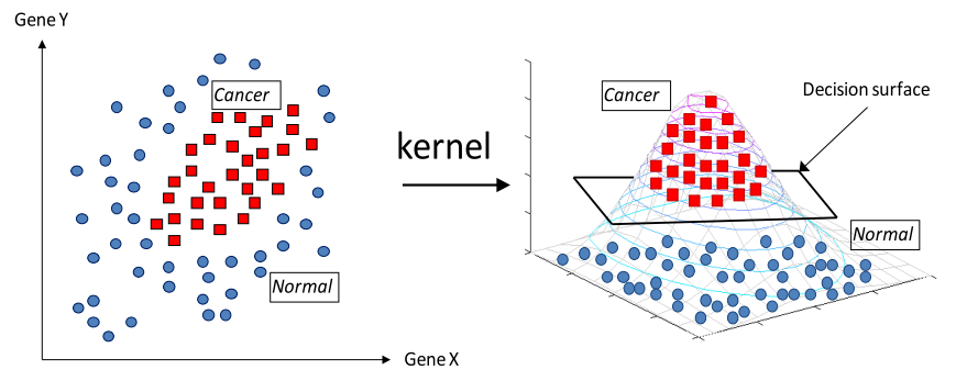
The kernel trick (like the RBF kernel) enables SVM to map non-linearly separable data into a higher-dimensional space, where it can be linearly separated.

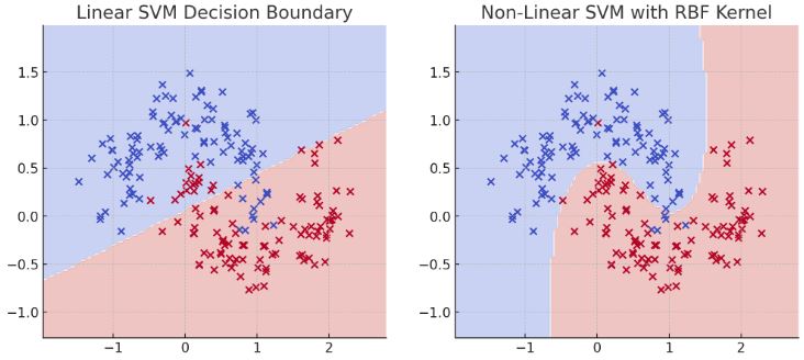
Another Example

• Left Plot (Linear SVM): The decision boundary is a straight line, which struggles to separate the moon-shaped clusters effectively.

• Right Plot (Non-Linear SVM with RBF Kernel): The decision boundary is curved, allowing the model to accurately separate the two classes.

5. Effect of Outliers

Outliers can significantly impact the performance of machine learning models, including logistic regression and Support Vector Machines (SVM). The effect of outliers on these models depends on the model specifics.

5.1 Logistic Regression and Outliers

Sensitivity

LR is quite sensitive to outliers, as LR tries to maximize the likelihood of the data when drawing the decision boundary. Thus an outliers that are far from ‘optimal’ decision boundar can pull it towards itself, leading to a skewed line.

Mitigation

• Regularization techniques, such as L1 and L2 regularization, can help mitigate the effect of outliers by penalizing large coefficients, thus reducing the sensitivity to outliers.
• Additionally, data-preprocessing steps such as outlier detection and removal can be helpful.

5.2 SVM and Outliers

Robustness

SVM tends to be more robust to outliers than logistic regression. This robustness comes from the fact that SVM focuses on maximizing the margin between the closest points of different classes (the support vectors) rather than fitting all the data points. As a result, as long as the outliers do not affect the position of the margin (i.e., they are not support vectors), their impact on the model will be limited.

Effect on Margin

However, if outliers are close to the decision boundary, they can become support vectors and affect the position of the margin. In cases where outliers are extreme and fall within the margin or on the wrong side of the decision boundary, they can significantly affect the SVM model by altering the margin and potentially causing misclassification of other instances.

Soft Margin SVM

The introduction of the soft margin SVM, which allows for some misclassifications (determined by the regularization parameter C), offers a way to control the influence of outliers. A lower value of C makes the model more tolerant to misclassifications (including those caused by outliers) and can help in reducing the impact of outliers on the decision boundary.

6. Multi-class Classification?

Logistic regression and SVM are naturally binary classifiers. But they can be extended for multi-class classification using two strategies: (you might need to draw an example to show them more intuitively)

6.1 One-vs-One (OvO)

• Strategy: In OvO, for a classification problem with classes, a binary classifier is trained for every pair of classes, resulting in classifiers in total. Each classifier is trained on data from two classes, determining which of the two it belongs to.

• Prediction: To make a prediction, all classifiers vote on the class. The class with the most votes is chosen as the final prediction.

• Advantages: OvO can be advantageous when the binary classification model scales poorly with the size of the training dataset because each classifier needs to be trained only on the subset of the data belonging to its two classes. It’s less sensitive to class imbalance compared to OvA.

• Disadvantages: The primary disadvantage of OvO is the computational cost in training and prediction time, as the number of classifiers grows quadratically with the number of classes.

One-vs-All (OvA) or One-vs-Rest (OvR)

• Strategy: In the OvA approach, one binary classifier is trained per class. For each classifier, the class it represents is treated as the positive class, and all other classes are combined into a single negative class. Therefore, for classes, separate classifiers are trained.

• Prediction: For a given input, each classifier predicts the probability that the input belongs to its class. The class corresponding to the classifier with the highest probability (or, in some implementations, the highest score or largest distance from the decision boundary) is selected as the final prediction.

• Advantages: OvA is conceptually simpler and computationally more efficient in terms of the number of classifiers needed compared to OvO, especially as the number of classes increases.

• Disadvantages: The main disadvantage of OvA is that each classifier is trained on the entire dataset, which can be less efficient if the binary classifier is particularly sensitive to the size of the training set. Additionally, OvA might struggle more with class imbalance since the negative class is a combination of all other classes.